Using Quarto
Quarto Markdown is regular Markdown with R code and output sprinkled in. You can do everything you can with regular Markdown, but you can incorporate graphs, tables, and other code output directly in your document. You can create HTML, PDF, and Word documents, PowerPoint and HTML presentations, websites, books, and even interactive dashboards with Quarto. This whole course website is created with Quarto.
Quarto’s predecessor was called R Markdown and worked exclusively with R (though there are ways to use other languages in document). Quarto is essentially “R Markdown 2.0,” but it is designed to be language agnostic. You can use R, Python, Julia, Observable JS, and even Stata code all in the same document. It is magical.
TipQuarto documentation
The documentation for Quarto is extremely comprehensive—rely on it throughout the semester! Here are some of the more important pages:
- Guide: A comprehensive guide to all the different things you can do with Quarto, including:
- Figures
- Tables
- Cross references
- Citations and footnotes
- Special layouts (like putting content in the margins)
- Callout blocks (like the green box this text is in)
- Reference: Complete documentation for all the options for specific formats, including these:
You can also use Quarto for books, websites, presentations, and dashboards.
Here are the most important things you’ll need to know about Quarto in this class:
Key terms
Document: A Markdown file where you type stuff
Chunk: A piece of R code that is included in your document. It looks like this:
```{r}
# Code goes here
1 + 1
```
There must be an empty line before and after the chunk. The final three backticks must be the only thing on the line—if you add more text, or if you forget to add the backticks, or accidentally delete the backticks, your document will not render correctly.
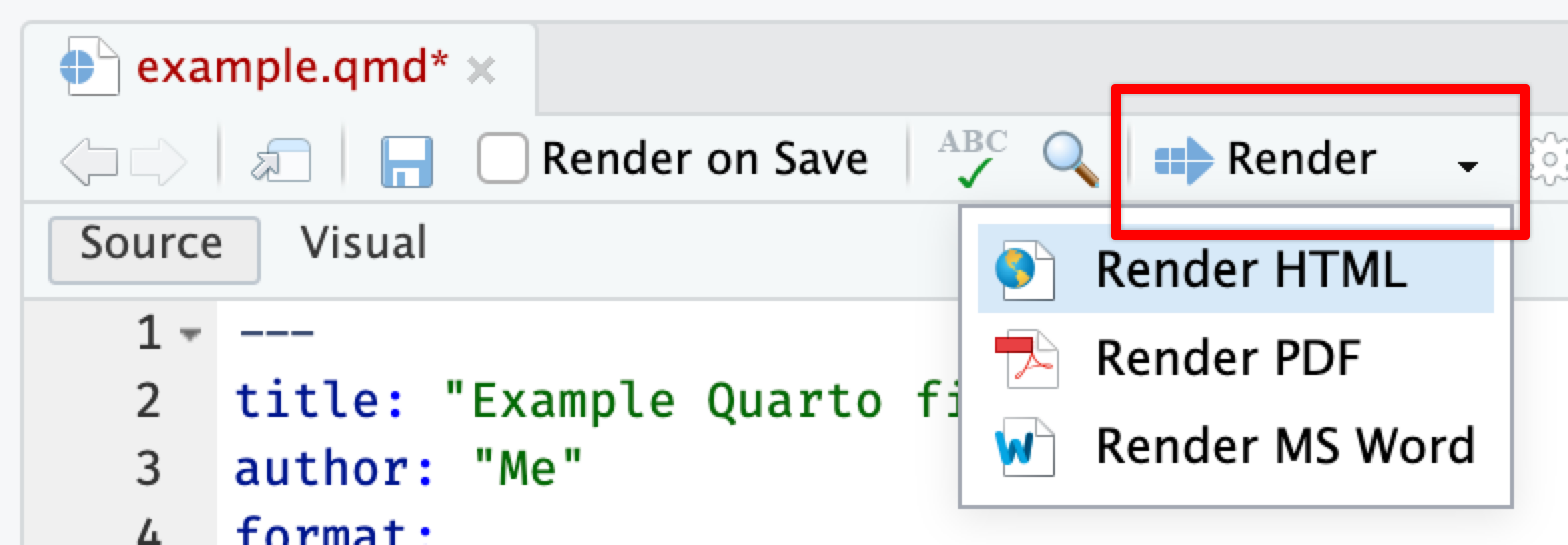
Render: When you render a document, R runs each of the chunks sequentially and converts the output of each chunk into Markdown. R then runs the document through pandoc to convert it to HTML or PDF or Word (or whatever output you’ve selected).
You can render by clicking on the “Render” button at the top of the editor window, or by pressing
⌘⇧Kon macOS orcontrol + shift + Kon Windows.
Add chunks
There are three ways to insert chunks:
Press
⌘⌥Ion macOS orcontrol + alt + Ion WindowsClick on the “Insert” button at the top of the editor window
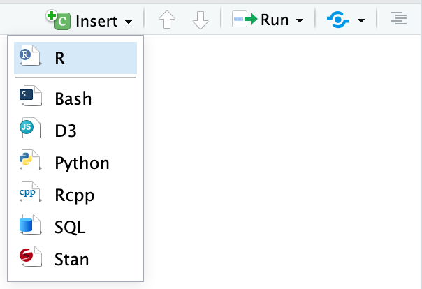
- Manually type all the backticks and curly braces (don’t do this)
Chunk names
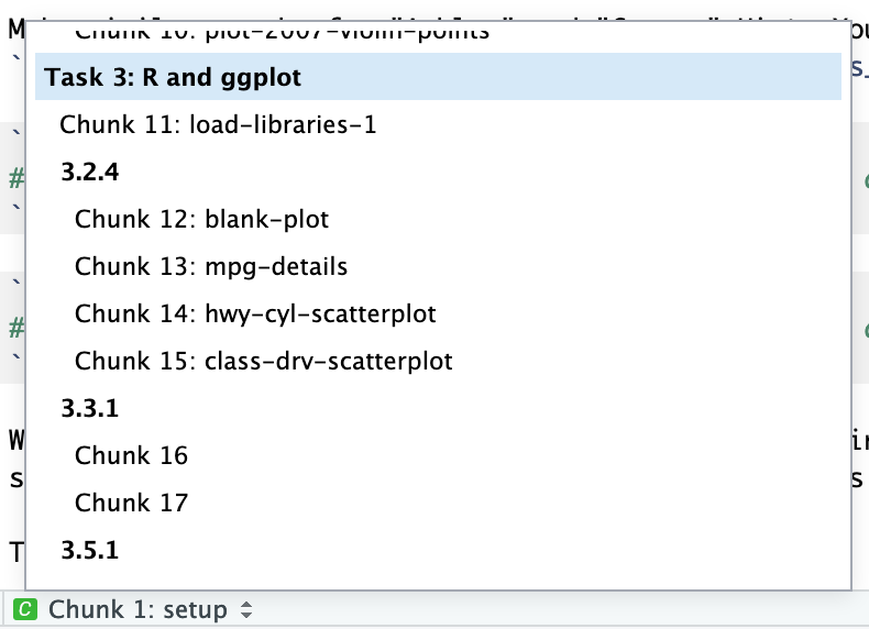
You can add names to chunks to make it easier to navigate your document. If you click on the little dropdown menu at the bottom of your editor in RStudio, you can see a table of contents that shows all the headings and chunks. If you name chunks, they’ll appear in the list. If you don’t include a name, the chunk will still show up, but you won’t know what it does.
There are two ways to add a chunk name:
As a special comment called
label:, following#|at the top of the chunk (this is the preferred way):```{r} #| label: name-of-this-chunk 1 + 1 ```Immediately after the
{rin the first line of the chunk (this is the older way):```{r name-of-this-chunk} 1 + 1 ```
Names cannot contain spaces, but they can contain underscores and dashes. All chunk names in your document must be unique.
Chunk options
There are a bunch of different options you can set for each chunk. You can see a complete list in the R Markdown Reference Guide or at {knitr}’s website.
Set chunk options as special comments following #| at the top of the chunk (this is the preferred way):
```{r}
#| label: fig-some-plot
#| fig-cap: "Here's a caption for this plot"
#| fig-width: 6
#| fig-height: 4
#| echo: false

ggplot(mpg, aes(x = displ, y = hwy, color = drv)) +
  geom_point() +
  geom_smooth(method = "lm")
```
Technically you can also set these options inside the {r} section of the chunk—this is the old way to do it, but it gets really gross and long when you have lots of settings:
{r fig-some-plot, fig.width=6, fig.height=4, echo=FALSE, fig.cap = "Here's a caption for this plot"}Here are some of the most common chunk options you’ll use in this class:
label: fig-whatever: Try to always use chunk labels. If you want things to be cross-referenceable, use afig-prefix on chunks that make figures and atbl-prefix on chunks that make tablestbl-cap: "Blah": Add a caption to your tablefig-cap: "Blah": Add a caption to your figurefig-width: 5andfig-height: 3(or whatever number you want): Set the dimensions for figuresecho: false: The code is not shown in the final document, but the results aremessage: false: Any messages that R generates (like all the notes that appear after you load a package) are omittedwarning: false: Any warnings that R generates are omittedinclude: false: The chunk still runs, but the code and results are not included in the final document
Inline chunks
You can also include R output directly in your text, which is really helpful if you want to report numbers from your analysis. To do this, use `r r_code_here`.
It’s generally easiest to calculate numbers in a regular chunk beforehand and then use an inline chunk to display the value in your text. For instance, this document…
```{{r}}
#| label: find-avg-mpg
#| echo: false
avg_mpg <- mean(mtcars$mpg)
```
The average fuel efficiency for cars from 1974 was r round(avg_mpg, 1) miles per gallon.
… would render to this:
The average fuel efficiency for cars from 1974 was 20.1 miles per gallon.
Output formats
You can specify what kind of document you create when you render in the YAML front matter.
title: "My document"
format:
  html: default
  pdf: default
  docx: default
The indentation of the YAML section matters, especially when you have settings nested under each output type. Here’s what a typical format section might look like:
---
title: "My document"
author: "My name"
date: "January 4, 2024"
format:
  html_document:
    toc: yes
  pdf_document:
    toc: yes
  word_document:
    toc: yes
---